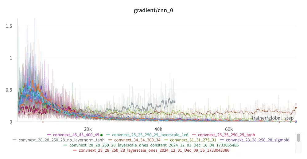
Mean gradient for 1st layer in all experiments
Introduction
One of the largest Convolutional Networks, ConvNext-XXLarge [1] from OpenCLIP[2], boasts approximately 850 million parameters and 120 layers (counting all convolutional and linear layers). This is a dramatic increase compared to the 8 layers of AlexNet[3] but still fewer than the 1001-layer experiment introduced in the PreResNet[4] paper.
Interestingly, about a decade ago, training networks with more than 100 layers was considered nearly impossible due to the vanishing gradient problem. However, advancements such as improved activation functions, normalization layers, and skip connections have significantly mitigated this issue or so it seems. But is the problem truly solved?
In this blog post, I will explore:
- What components enable training neural networks with more than 1,000 layers?
- Is it possible to train a 10,000-layer Convolutional Neural Network successfully?
Vanishing gradient issue
Before diving into experiments, lets briefly revisit the vanishing gradient problem , a challenge that many sources have already explored in detail.
The vanishing gradient problem occurs when the gradients in the early layers of a neural network become extremely small, effectively halting their ability to learn useful features. This issue arises due to the chain rule used during backpropagation, where the gradient is propagated backward from the final layer to the first. If the gradient in any layer is close to zero, the gradients for preceding layers shrink exponentially. A major cause of this behavior is the saturation of activation functions.
To illustrate this, I trained a simple 5-layer network using the sigmoid activation function, which is particularly prone to saturation. You can find the code for this experiment on GitHub. The goal was to observe how the gradient norms of the networks weights evolve over time.

Gradient Norms Per Layer (Vanishing Gradient Issue). FC5 is the top layer, FC1 is the first layer. Image by author
The plot above shows the gradient norms for each linear layer over several training iterations. FC5 represents the final layer, while FC1 represents the first.
Vanishing Gradient Problem:
- In the first training iteration, theres a huge difference in gradient norms between FC5 and FC4, with FC4 being approximately 10x smaller.
- By the time we reach FC1, the gradient is reduced by a factor of ~10,000 compared to FC5, leaving almost nothing of the original gradient to update the weights.
This is a textbook example of the vanishing gradient problem, primarily driven by activation function saturation.
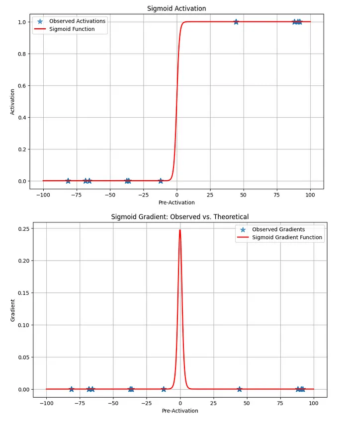
Sigmoid activation function and its gradient. Plot add preactivation and activations/gradient values. Image by author
Lets delve deeper into the root cause: the sigmoid activation function. To understand its impact, I analyzed the first layer’s pre-activation values (inputs to the sigmoid). The findings:
- Most pre-activation values lie in the flat regions of the sigmoid curve, resulting in activations close to 0 or 1.
- In these regions, the sigmoid gradient is nearly zero, as shown in the plot above.
This means that any gradient passed backward through these layers is severely diminished, effectively disappearing by the time it reaches the first layers.The maximum gradient of the sigmoid function is 0.25 , achieved at the midpoint of the curve. Even under ideal conditions, with 5 layers, the maximum gradient diminishes to 0.25 1e-3. This reduction becomes catastrophic for networks with 1,000 layers, rendering negligible the first layers’ gradients.
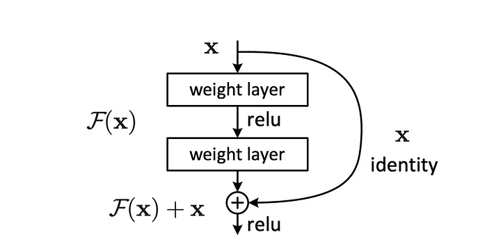
Skip connection. Source: Deep Residual Learning for Image Recognition, Kaiming He
Mitigation of the vanishing gradient issue
Several advancements have been instrumental in addressing the vanishing gradient problem, making it possible to train very deep neural networks. The key components that contribute to this solution are:
1. Activation Functions (e.g., Tanh, ReLU, GeLU)
Modern activation functions have been designed to mitigate vanishing gradients by offering higher maximum gradient values and reducing regions where the gradient is zero. For example:
- ReLU (Rectified Linear Unit) has a maximum gradient of 1.0 and eliminates the saturation problem for positive inputs. This ensures gradients remain significant during backpropagation.
- Other functions, such as GeLU [5] and Swish [6], smooth out the gradient landscape, further improving training stability.
2. Normalization Techniques (e.g., BatchNorm [7] , LayerNorm [8] )
Normalization layers play a crucial role by adjusting pre-activation values to have a mean close to zero and a consistent variance. This helps in two significant ways:
- It reduces the likelihood of pre-activation values entering the saturation regions of activation functions, where gradients are nearly zero.
- Normalization ensures more stable training by keeping the activations well-distributed across layers.
For instance:
- BatchNorm [7] normalizes the input to each layer based on the batch statistics during training.
- LayerNorm [8] normalizes across features for each sample, making it more effective in some scenarios.
3. Skip Connections (Residual Connections)
Skip connections, introduced in architectures like ResNet[9], allow input signals to bypass one or more intermediate layers by directly adding the input to the layer’s output. This mechanism addresses the vanishing gradient problem by:
- Providing a direct pathway for gradients to flow back to earlier layers without being multiplied by small derivatives or passed through saturating activation functions.
- Preserving gradients even in very deep networks, ensuring effective learning for earlier layers.
By avoiding multiplications or transformations in the skip path, gradients remain intact, making them a simple yet powerful tool for training ultra-deep networks.

Skip connection equation. Image by author
Training 1000 layer network
For this experiment, all training was conducted on the CIFAR-10 [10] dataset. The baseline architecture was ConvNext[1] , chosen for its scalability and effectiveness in modern vision tasks. To define successful convergence, I used a validation accuracy of >50% (compared to the 10% accuracy of random guessing). Source code on GitHub. All runs are available at Wandb.
The following parameters were used across all experiments:
- Batch size: 64
- Optimizer: AdamW[11]
- Learning rate scheduler: OneCycleLR
My primary objective was to replicate the findings of the PreResNet paper and investigate how adding more layers impacts training. Starting with a 26-layer network as the baseline, I gradually increased the number of layers, ultimately reaching 1,004 layers.
Throughout the training process, I collected statistics on the mean absolute gradient of the first convolutional layer. This allowed me to evaluate how effectively gradients propagated back through the network as the depth increased.

Training 1k layer experiments. Image by author
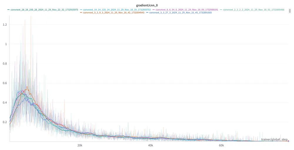
Gradient plot for all experiments. Despite the depth, gradient at the first layer are similar in each run. Image by author
Key Observations
- Despite increasing the depth to 1,000 layers, the networks successfully converged, consistently achieving the validation accuracy threshold (>50%).
- The mean absolute gradient of the first layer remained sufficiently large across all tested depths, indicating effective gradient propagation even in the deepest networks.
- The scores of ~94% are weak as SOTA is ~99%. I couldnt get better scores, leaving space for the next investigations.
Training component analysis
Before diving deeper into ultra-deep networks, its crucial to identify which components most significantly impact the ability to train a 1000-layer network. The candidates are:
- Activation functions
- Normalization layers
- Skip connections
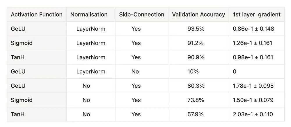
Training component analysis experiments. Image by author
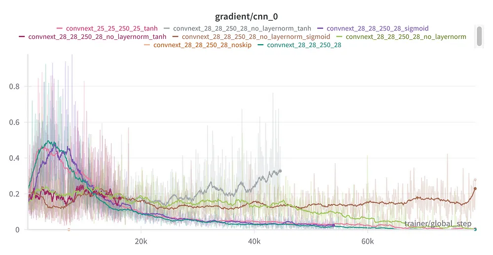
Gradient plot for training component analysis experiments. . Image by author
Skip Connections: The Clear Winner
Among all components, skip connections stand out as the most critical factor. Without skip connections, no other modifications advanced activation functions or normalization techniques can sustain training for such deep networks. This confirms that skip connections are the cornerstone of vanishing gradient mitigation.
Activation Functions: Sigmoid and Tanh Still Competitive
Surprisingly, the performance of Sigmoid and Tanh activation functions was competitive with modern alternatives like GeLU when accompanied by the normalization layer, and even without LayerNorm Sigmoid got a competitive score compared to GELU without LayerNorm. As we see, the mean gradient for all experiments is quite similar, with TanH without LayerNorm having the highest mean value but at the same time the lowest accuracy.
Mean Gradient Values
The mean gradient values are relatively consistent across experiments, but the gradient trajectories differ. In experiments with LayerNorm, gradients initially rise to approximately 0.5 early in training before steadily declining. In contrast, experiments without LayerNorm exhibit a nearly constant gradient throughout the training process. Importantly, the gradient remains present in all cases, with no evidence of vanishing gradients in the networks first layer.
Diving Deeper into Skip Connections
Skip connections can be implemented in various ways, with the main difference being how the raw input and transformed output are merged, often controlled by a learnable scaling factor ****. In ConvNext, for instance, the LayerScale [12] trick is employed, where the transformed data is scaled by a small learnable , initialized to 1e-6.
This setup has a profound implication:
- During the initial training stages, most information flows through the skip connections, as the contribution from the transformation branch (via matrix multiplication and activation functions) is minimal.
- As a result, the vanishing gradient issue is effectively bypassed.

Skip connection in ConvNext, with **** symbol. Image by author
Experiment: Varying LayerScale Initialization
To test whether the initialization of plays a critical role, I experimented with different starting values for LayerScale. Below is a diagram of a typical skip connection and a table summarizing the results:
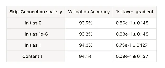
Skip connection scale analysis experiments. Image by author
The results show that even with initialized to 1 (effectively turning on all transformation branches from the start), training a 1000-layer network remained stable. This suggests that while different versions of skip connections may vary slightly in their implementation, all are equally effective at mitigating the vanishing gradient problem.
> 1000-layer network
Since weve established that skip connections are the key to training very deep networks, lets push the limits further by experimenting with even deeper architectures. To do this, I will gradually increase the network depth, but deeper networks require significantly more computational resources. Therefore, Ive decided to fit the largest possible network that can run on an RTX 4090 with 24 GB of memory.

Fitting the biggest possible network on 24 GB. Image by author.
The 1607-layer ConvNext was the biggest one I could fit into a GPU memory. There is still no issue with convergence, and the CIFAR10 results are the same.
Summary
To sum up a key finding:
- the skip connection is a main vanishing gradient mitigation tool
- Tanh/Sigmoid are competitive to GELU when used with skip-connection and LayerNorm. It means that despite flat gradient areas Tanh/Sigmoid works well when accompanied by Skip-Connection and LayerNorm
- with skip-connection, you can try any depth you want, only resources constrain you, no matter what activation function you choose
If anybody does not agree with that thesis during the recruitment process, send the link to my blog post as my experiment shows clear evidence!
[1] A ConvNet for the 2020s, Zhuang Liu, CVPR 2022
[2] OpenCLIP, Ross Wightman, Romain Beaumont, Cade Gordon, Vaishaal Shankar, 2021
[3] ImageNet Classification with Deep Convolutional Neural Networks, Alex Krizhevsky, NIPS 2012
[4] Identity Mappings in Deep Residual Networks, Kaiming He, ECCV 2016
[5] Gaussian Error Linear Units, Dan Hendrycks, 2016
[6] Searching for Activation Functions, Prajit Ramachandran, ICLR 2018
[7] Batch Normalization: Accelerating Deep Network Training by Reducing Internal Covariate Shift, Sergey Ioffe, ICML 2015
[8] Layer Normalization, Jimmy Lei Ba, 2016
[9] Deep Residual Learning for Image Recognition, Kaiming He, CVPR 2016
[10] Learning Multiple Layers of Features from Tiny Images, Alex Krizhevsky, 2009
[11] Decoupled Weight Decay Regularization, Ilya Loshchilov, ICLR 2019
[12] Going deeper with Image Transformers, Hugo Touvron, ICCV 2021

