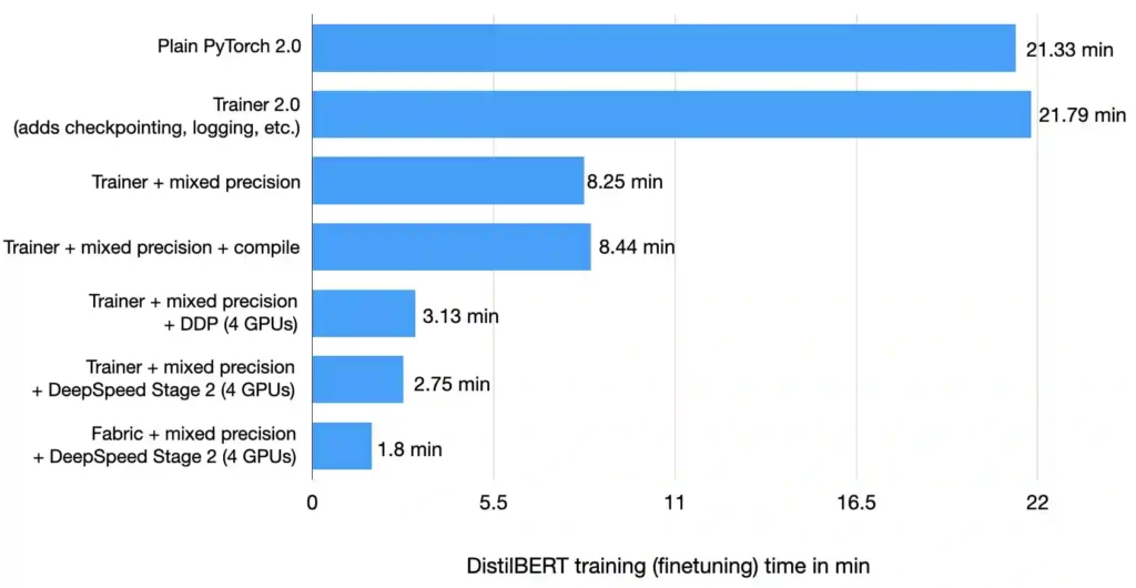
This blog post outlines techniques for improving the training performance of your PyTorch model without compromising its accuracy. To do so, we will wrap a PyTorch model in a LightningModule and use the Trainer class to enable various training optimizations. By changing only a few lines of code, we can reduce the training time on a single GPU from 22.53 minutes to 2.75 minutes while maintaining the model’s prediction accuracy.
Yes, that’s a 8x performance boost!

(This blog post was updated on 03/17/2023, now using PyTorch 2.0 and Lightning 2.0!)
Introduction
In this tutorial, we will finetune a DistilBERT model, a distilled version of BERT that is 40% smaller at almost identical predictive performance. There are several ways we can finetune a pretrained language model. The figure below depicts the three most common approaches.
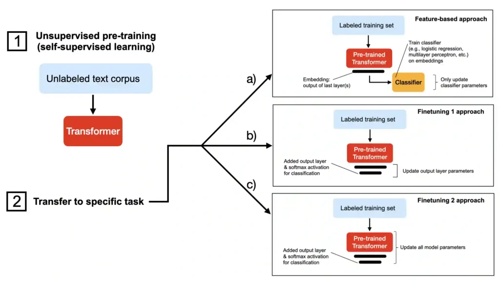
All three approaches above (a-c) assume we have pretrained the model on an unlabeled dataset using self-supervised learning. Then, in step 2, when we transfer the model to the target task, we either
- a) extract the embeddings and train a classifier on these (this can be a support vector machine from scikit-learn, for example);
- b) replace/add an output layer and finetune the last layer(s) of the transformer;
- c) replace/add an output layer and finetune all layers.
The approaches a-c are ordered by computational efficiency, where a) is typically the fastest. In my experience, this sorting order also reflects the model’s predictive performance, where c) usually yields the highest prediction accuracy.
In this tutorial, we will use approach c) and train a model to predict the sentiment of movie reviews in the IMDB Large Movie Review dataset consisting of 50,000 movie reviews in total.
1) Plain PyTorch Baseline
As a warm-up exercise, let’s start with the plain PyTorch baseline for training the DistilBERT model on the IMDB movie review dataset. If you want to run the code yourself, you can set up a virtual environment with the relevant Python libraries as follows:
    conda create -n faster-blog python=3.9
    conda activate faster-blog

    pip install watermark transformers datasets torchmetrics lightning
For reference, the relevant software versions I was using are the following (they will be printed to the terminal when you run the code later in this article.):
    Python version: 3.9.15
    torch         : 2.0.0+cu118
    lightning     : 2.0.0
    transformers  : 4.26.1
To avoid bloating this article with boring data-loading utilities, I will skip over the local_dataset_utilities.py file, which contains code to load the dataset. The only relevant information here is that we are partitioning the dataset into 35,000 training examples, 5,000 validation set records, and 10,000 test records.
Let’s get to the main PyTorch code. This code is self-contained except for the dataset loading utilities I placed in the local_dataset_utilities.py file. Have a look at the PyTorch code before we discuss it below:
    import os
    import os.path as op
    import time

    from datasets import load_dataset
    import torch
    from torch.utils.data import DataLoader
    import torchmetrics
    from transformers import AutoTokenizer
    from transformers import AutoModelForSequenceClassification
    from watermark import watermark

    from local_dataset_utilities import (
        download_dataset,
        load_dataset_into_to_dataframe,
        partition_dataset,
    )
    from local_dataset_utilities import IMDBDataset


    def tokenize_text(batch):
        return tokenizer(batch["text"], truncation=True, padding=True)


    def train(num_epochs, model, optimizer, train_loader, val_loader, device):
        for epoch in range(num_epochs):
            train_acc = torchmetrics.Accuracy(task="multiclass", num_classes=2).to(device)

            for batch_idx, batch in enumerate(train_loader):
                model.train()
                for s in ["input_ids", "attention_mask", "label"]:
                    batch[s] = batch[s].to(device)

                ### FORWARD AND BACK PROP
                outputs = model(
                    batch["input_ids"],
                    attention_mask=batch["attention_mask"],
                    labels=batch["label"],
                )
                optimizer.zero_grad()
                outputs["loss"].backward()

                ### UPDATE MODEL PARAMETERS
                optimizer.step()

                ### LOGGING
                if not batch_idx % 300:
                    print(
                        f"Epoch: {epoch+1:04d}/{num_epochs:04d} | Batch {batch_idx:04d}/{len(train_loader):04d} | Loss: {outputs['loss']:.4f}"
                    )

                model.eval()
                with torch.no_grad():
                    predicted_labels = torch.argmax(outputs["logits"], 1)
                    train_acc.update(predicted_labels, batch["label"])

            ### MORE LOGGING
            with torch.no_grad():
                model.eval()
                val_acc = torchmetrics.Accuracy(task="multiclass", num_classes=2).to(device)
                for batch in val_loader:
                    for s in ["input_ids", "attention_mask", "label"]:
                        batch[s] = batch[s].to(device)
                    outputs = model(
                        batch["input_ids"],
                        attention_mask=batch["attention_mask"],
                        labels=batch["label"],
                    )
                    predicted_labels = torch.argmax(outputs["logits"], 1)
                    val_acc.update(predicted_labels, batch["label"])

                print(
                    f"Epoch: {epoch+1:04d}/{num_epochs:04d} | Train acc.: {train_acc.compute()*100:.2f}% | Val acc.: {val_acc.compute()*100:.2f}%"
                )


        print(watermark(packages="torch,lightning,transformers", python=True))
        print("Torch CUDA available?", torch.cuda.is_available())
        device = "cuda:0" if torch.cuda.is_available() else "cpu"

        torch.manual_seed(123)

        ##########################
        ### 1 Loading the Dataset
        ##########################
        download_dataset()
        df = load_dataset_into_to_dataframe()
        if not (op.exists("train.csv") and op.exists("val.csv") and op.exists("test.csv")):
            partition_dataset(df)

        imdb_dataset = load_dataset(
            "csv",
            data_files={
                "train": "train.csv",
                "validation": "val.csv",
                "test": "test.csv",
            },
        )

        #########################################
        ### 2 Tokenization and Numericalization
        #########################################

        tokenizer = AutoTokenizer.from_pretrained("distilbert-base-uncased")
        print("Tokenizer input max length:", tokenizer.model_max_length, flush=True)
        print("Tokenizer vocabulary size:", tokenizer.vocab_size, flush=True)

        print("Tokenizing ...", flush=True)
        imdb_tokenized = imdb_dataset.map(tokenize_text, batched=True, batch_size=None)
        del imdb_dataset
        imdb_tokenized.set_format("torch", columns=["input_ids", "attention_mask", "label"])
        os.environ["TOKENIZERS_PARALLELISM"] = "false"

        #########################################
        ### 3 Set Up DataLoaders
        #########################################

        train_dataset = IMDBDataset(imdb_tokenized, partition_key="train")
        val_dataset = IMDBDataset(imdb_tokenized, partition_key="validation")
        test_dataset = IMDBDataset(imdb_tokenized, partition_key="test")

        train_loader = DataLoader(
            dataset=train_dataset,
            batch_size=12,
            shuffle=True,
            num_workers=1,
            drop_last=True,
        )

        val_loader = DataLoader(
            dataset=val_dataset,
            batch_size=12,
            num_workers=1,
            drop_last=True,
        )

        test_loader = DataLoader(
            dataset=test_dataset,
            batch_size=12,
            num_workers=1,
            drop_last=True,
        )

        #########################################
        ### 4 Initializing the Model
        #########################################

        model = AutoModelForSequenceClassification.from_pretrained(
            "distilbert-base-uncased", num_labels=2
        )

        model.to(device)
        optimizer = torch.optim.Adam(model.parameters(), lr=5e-5)

        #########################################
        ### 5 Finetuning
        #########################################

        start = time.time()
        train(
            num_epochs=3,
            model=model,
            optimizer=optimizer,
            train_loader=train_loader,
            val_loader=val_loader,
            device=device,
        )

        end = time.time()
        elapsed = end - start
        print(f"Time elapsed {elapsed/60:.2f} min")

        with torch.no_grad():
            model.eval()
            test_acc = torchmetrics.Accuracy(task="multiclass", num_classes=2).to(device)
            for batch in test_loader:
                for s in ["input_ids", "attention_mask", "label"]:
                    batch[s] = batch[s].to(device)
                outputs = model(
                    batch["input_ids"],
                    attention_mask=batch["attention_mask"],
                    labels=batch["label"],
                )
                predicted_labels = torch.argmax(outputs["logits"], 1)
                test_acc.update(predicted_labels, batch["label"])

        print(f"Test accuracy {test_acc.compute()*100:.2f}%")
(You can also find this code on GitHub here: 1_pytorch-distilbert.py.)
To keep this article focused, I will skip over the PyTorch basics and focus on describing the main outline of this script. However, if you are new to PyTorch, I recommend checking out my free Deep Learning Fundamentals course, where I teach PyTorch in great detail in Units 1-4.
The code above is structured into two parts, the function definitions and the code executed under if __name__ == "__main__". This recommended structure is necessary to avoid issues with Python’s multiprocessing when using multiple GPUs later.
The first three sections of the if __name__ == "__main__" part contain the code to set up the dataset loaders. The fourth part is where we initialize the model: a pretrained DistilBERT model we will finetune. Then, in the fifth part, we run our training function and evaluate the finetuned model on the test set.
After running the code on an A100 GPU, I got the following results:
    Epoch: 0001/0003 | Batch 0000/2916 | Loss: 0.6867
    Epoch: 0001/0003 | Batch 0300/2916 | Loss: 0.3633
    Epoch: 0001/0003 | Batch 0600/2916 | Loss: 0.4122
    Epoch: 0001/0003 | Batch 0900/2916 | Loss: 0.3046
    Epoch: 0001/0003 | Batch 1200/2916 | Loss: 0.3859
    Epoch: 0001/0003 | Batch 1500/2916 | Loss: 0.4489
    Epoch: 0001/0003 | Batch 1800/2916 | Loss: 0.5721
    Epoch: 0001/0003 | Batch 2100/2916 | Loss: 0.6470
    Epoch: 0001/0003 | Batch 2400/2916 | Loss: 0.3116
    Epoch: 0001/0003 | Batch 2700/2916 | Loss: 0.2002
    Epoch: 0001/0003 | Train acc.: 89.81% | Val acc.: 92.17%
    Epoch: 0002/0003 | Batch 0000/2916 | Loss: 0.0935
    Epoch: 0002/0003 | Batch 0300/2916 | Loss: 0.0674
    Epoch: 0002/0003 | Batch 0600/2916 | Loss: 0.1279
    Epoch: 0002/0003 | Batch 0900/2916 | Loss: 0.0686
    Epoch: 0002/0003 | Batch 1200/2916 | Loss: 0.0104
    Epoch: 0002/0003 | Batch 1500/2916 | Loss: 0.0888
    Epoch: 0002/0003 | Batch 1800/2916 | Loss: 0.1151
    Epoch: 0002/0003 | Batch 2100/2916 | Loss: 0.0648
    Epoch: 0002/0003 | Batch 2400/2916 | Loss: 0.0656
    Epoch: 0002/0003 | Batch 2700/2916 | Loss: 0.0354
    Epoch: 0002/0003 | Train acc.: 95.02% | Val acc.: 92.09%
    Epoch: 0003/0003 | Batch 0000/2916 | Loss: 0.0143
    Epoch: 0003/0003 | Batch 0300/2916 | Loss: 0.0108
    Epoch: 0003/0003 | Batch 0600/2916 | Loss: 0.0228
    Epoch: 0003/0003 | Batch 0900/2916 | Loss: 0.0140
    Epoch: 0003/0003 | Batch 1200/2916 | Loss: 0.0220
    Epoch: 0003/0003 | Batch 1500/2916 | Loss: 0.0123
    Epoch: 0003/0003 | Batch 1800/2916 | Loss: 0.0495
    Epoch: 0003/0003 | Batch 2100/2916 | Loss: 0.0039
    Epoch: 0003/0003 | Batch 2400/2916 | Loss: 0.0168
    Epoch: 0003/0003 | Batch 2700/2916 | Loss: 0.1293
    Epoch: 0003/0003 | Train acc.: 97.28% | Val acc.: 89.88%
    Time elapsed 21.33 min
    Test accuracy 89.92%
As we can see above, the model starts overfitting slightly from epochs 2 to 3, and the validation accuracy decreased from 92.09% to 89.88%. The final test accuracy is 89.92%, which we reached after finetuning the model for 21.33 min.
2) Using the Trainer Class
Now, let’s wrap our PyTorch model in a LightningModule so that we can use the Trainer class from Lightning:
    import os
    import os.path as op
    import time

    from datasets import load_dataset
    import lightning as L
    from lightning.pytorch.callbacks import ModelCheckpoint
    from lightning.pytorch.loggers import CSVLogger
    import matplotlib.pyplot as plt
    import pandas as pd
    import torch
    from torch.utils.data import DataLoader
    import torchmetrics
    from transformers import AutoTokenizer
    from transformers import AutoModelForSequenceClassification
    from watermark import watermark

    from local_dataset_utilities import (
        download_dataset,
        load_dataset_into_to_dataframe,
        partition_dataset,
    )
    from local_dataset_utilities import IMDBDataset


    def tokenize_text(batch):
        return tokenizer(batch["text"], truncation=True, padding=True)

    class LightningModel(L.LightningModule):
        def __init__(self, model, learning_rate=5e-5):
            super().__init__()

            self.learning_rate = learning_rate
            self.model = model

            self.train_acc = torchmetrics.Accuracy(task="multiclass", num_classes=2)
            self.val_acc = torchmetrics.Accuracy(task="multiclass", num_classes=2)
            self.test_acc = torchmetrics.Accuracy(task="multiclass", num_classes=2)

        def forward(self, input_ids, attention_mask, labels):
            return self.model(input_ids, attention_mask=attention_mask, labels=labels)

        def training_step(self, batch, batch_idx):
            outputs = self(
                batch["input_ids"],
                attention_mask=batch["attention_mask"],
                labels=batch["label"],
            )
            self.log("train_loss", outputs["loss"])
            with torch.no_grad():
                logits = outputs["logits"]
                predicted_labels = torch.argmax(logits, 1)
                self.train_acc(predicted_labels, batch["label"])
                self.log("train_acc", self.train_acc, on_epoch=True, on_step=False)
            return outputs["loss"]  # this is passed to the optimizer for training

        def validation_step(self, batch, batch_idx):
            outputs = self(
                batch["input_ids"],
                attention_mask=batch["attention_mask"],
                labels=batch["label"],
            )
            self.log("val_loss", outputs["loss"], prog_bar=True)

            logits = outputs["logits"]
            predicted_labels = torch.argmax(logits, 1)
            self.val_acc(predicted_labels, batch["label"])
            self.log("val_acc", self.val_acc, prog_bar=True)

        def test_step(self, batch, batch_idx):
            outputs = self(
                batch["input_ids"],
                attention_mask=batch["attention_mask"],
                labels=batch["label"],
            )

            logits = outputs["logits"]
            predicted_labels = torch.argmax(logits, 1)
            self.test_acc(predicted_labels, batch["label"])
            self.log("accuracy", self.test_acc, prog_bar=True)

        def configure_optimizers(self):
            optimizer = torch.optim.Adam(
                self.trainer.model.parameters(), lr=self.learning_rate
            )
            return optimizer


    if __name__ == "__main__":
        print(watermark(packages="torch,lightning,transformers", python=True), flush=True)
        print("Torch CUDA available?", torch.cuda.is_available(), flush=True)

        torch.manual_seed(123)

        ##########################
        ### 1 Loading the Dataset
        ##########################
        download_dataset()
        df = load_dataset_into_to_dataframe()
        if not (op.exists("train.csv") and op.exists("val.csv") and op.exists("test.csv")):
            partition_dataset(df)

        imdb_dataset = load_dataset(
            "csv",
            data_files={
                "train": "train.csv",
                "validation": "val.csv",
                "test": "test.csv",
            },
        )

        #########################################
        ### 2 Tokenization and Numericalization
        ########################################

        tokenizer = AutoTokenizer.from_pretrained("distilbert-base-uncased")
        print("Tokenizer input max length:", tokenizer.model_max_length, flush=True)
        print("Tokenizer vocabulary size:", tokenizer.vocab_size, flush=True)

        print("Tokenizing ...", flush=True)
        imdb_tokenized = imdb_dataset.map(tokenize_text, batched=True, batch_size=None)
        del imdb_dataset
        imdb_tokenized.set_format("torch", columns=["input_ids", "attention_mask", "label"])
        os.environ["TOKENIZERS_PARALLELISM"] = "false"

        #########################################
        ### 3 Set Up DataLoaders
        #########################################

        train_dataset = IMDBDataset(imdb_tokenized, partition_key="train")
        val_dataset = IMDBDataset(imdb_tokenized, partition_key="validation")
        test_dataset = IMDBDataset(imdb_tokenized, partition_key="test")

        train_loader = DataLoader(
            dataset=train_dataset,
            batch_size=12,
            shuffle=True,
            num_workers=1,
            drop_last=True,
        )

        val_loader = DataLoader(
            dataset=val_dataset,
            batch_size=12,
            num_workers=1,
            drop_last=True,
        )

        test_loader = DataLoader(
            dataset=test_dataset,
            batch_size=12,
            num_workers=1,
            drop_last=True,
        )

        #########################################
        ### 4 Initializing the Model
        #########################################

        model = AutoModelForSequenceClassification.from_pretrained(
            "distilbert-base-uncased", num_labels=2
        )

        #########################################
        ### 5 Finetuning
        #########################################

        lightning_model = LightningModel(model)

        callbacks = [
            ModelCheckpoint(save_top_k=1, mode="max", monitor="val_acc")  # save top 1 model
        ]
        logger = CSVLogger(save_dir="logs/", name="my-model")

        trainer = L.Trainer(
            max_epochs=3,
            callbacks=callbacks,
            accelerator="gpu",
            devices=[1],
            logger=logger,
            log_every_n_steps=10,
            deterministic=True,
        )

        start = time.time()
        trainer.fit(
            model=lightning_model,
            train_dataloaders=train_loader,
            val_dataloaders=val_loader,
        )

        end = time.time()
        elapsed = end - start
        print(f"Time elapsed {elapsed/60:.2f} min")

        test_acc = trainer.test(lightning_model, dataloaders=test_loader, ckpt_path="best")
        print(test_acc)

        with open(op.join(trainer.logger.log_dir, "outputs.txt"), "w") as f:
            f.write((f"Time elapsed {elapsed/60:.2f} min\n"))
            f.write(f"Test acc: {test_acc}")
(You can also find this code on GitHub here: 2_pytorch-with-trainer.py.)
Again, I am skipping the details of the LightningModule to keep this article focused on the performance aspects. However, I will cover the LightningModule and Trainer classes in more detail in Unit 5 of my Deep Learning Fundamentals course, which is set to come out in March. In the meantime, I recommend the official PyTorch Lightning tutorial.
In short, we set up a LightningModule that defines how a training, validation, and test step is executed. Then, the main change is in the code section 5, where we finetune the model. What’s new is that we are now wrapping the PyTorch model in the LightningModel class and using the Trainer class to fit the model:
        #########################################
        ### 5 Finetuning
        #########################################

        lightning_model = LightningModel(model)

        callbacks = [
            ModelCheckpoint(save_top_k=1, mode="max", monitor="val_acc")  # save top 1 model
        ]
        logger = CSVLogger(save_dir="logs/", name="my-model")

        trainer = L.Trainer(
            max_epochs=3,
            callbacks=callbacks,
            accelerator="gpu",
            devices=1,
            logger=logger,
            log_every_n_steps=10,
            deterministic=True,
        )

        trainer.fit(
            model=lightning_model,
            train_dataloaders=train_loader,
            val_dataloaders=val_loader,
        )
Since we previously noticed that the validation accuracy decreases from epoch 2 to 3, we use a ModelCheckpoint callback to load the best model (based on the highest validation accuracy) for model evaluation on the test set. Moreover, we will log the performance to a CSV file (my preferred method for record-keeping) and set the PyTorch behavior to deterministic.
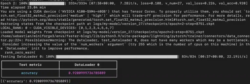
On the same machine, this model reached a test accuracy of 92.6% in 21.79 min:
Note that if we disable checkpointing and allow PyTorch to run in non-deterministic mode, we would get the same runtime as will plain PyTorch.
3) Automatic Mixed Precision Training
If our GPU supports mixed precision training, enabling it is often one of the main ways to boost computational efficiency. In particular, we use automatic mixed precision training, which switches between 32-bit and 16-bit floating point representations during training without sacrificing accuracy.
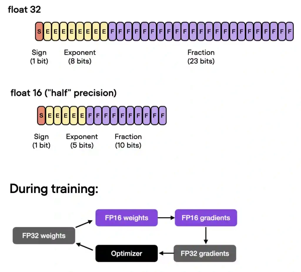
Using the Trainer class, we can enable automatic mixed precision training with one line of code:
        trainer = L.Trainer(
            max_epochs=3,
            callbacks=callbacks,
            accelerator="gpu",
            precision="16",  # <-- NEW
            devices=[1],
            logger=logger,
            log_every_n_steps=10,
            deterministic=True,
        )
Using mixed precision training, as shown above, boosts the training time from 21.79 min to 8.25 min! That’s almost 3x faster!
The test set accuracy is 93.2% – even slightly improved compared to the 92.6% before (likely due to rounding-induced differences when switching between the different precision modes.)

4) Static Graphs with Torch.Compile
In the recent PyTorch 2.0 announcement, the PyTorch team introduced the new toch.compile function that can speed up PyTorch code execution by generating optimized static graphs instead of running PyTorch code with dynamic graphs (the so-called eager mode). Under the hood, this is a 3-step process including graph acquisition, graph lowering, and graph compilation.
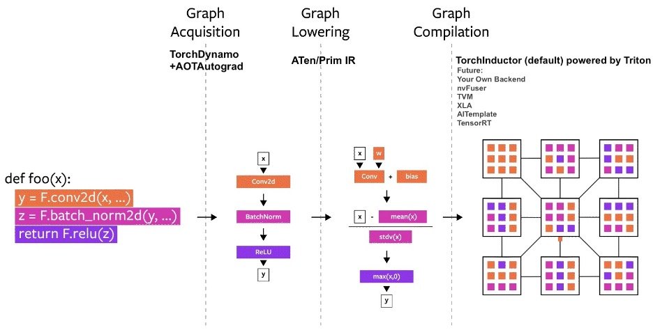
(Image source: https://pytorch.org/get-started/pytorch-2.0/)
There are lots of sophisticated things under the hood that make this happen, which are explained in more detail in the PyTorch 2.0 announcement. As a user, we can use this new feature via one simple command, torch.compile.
To take advantage of torch.compile, we can modify our code by adding this one-liner:
    # ...
    model = AutoModelForSequenceClassification.from_pretrained(
            "distilbert-base-uncased", num_labels=2
        )

    model = torch.compile(model) # NEW
    lightning_model = LightningModel(model)
    # ...
(For more details on the torch.compile function, please also see the official torch.compile tutorial)
Unfortunately, it seems that torch.compile does not result in a performance boost for DistilBERT model in this mixed-precision context when using the default parameters. The training time was 8.44 min, compared to 8.25 min before. So, the followin benchmarks in this tutorial will not be using torch.compile.

Sidenote: when applyting two tricks,
- placing the compilation before the timing starts;
- priming the model with an example batch as shown below
      model.to(torch.device("cuda:0"))
      model = torch.compile(model)

      for batch_idx, batch in enumerate(train_loader):
          model.train()
          for s in ["input_ids", "attention_mask", "label"]:
              batch[s] = batch[s].to(torch.device("cuda:0"))
          break

      outputs = model(
          batch["input_ids"],
          attention_mask=batch["attention_mask"],
          labels=batch["label"],
      )

      lightning_model = LightningModel(model)
      # start timing and training below
the runtime improves to 5.6 min. This indicates that the initial optimization compilation step takes a few minutes but eventually accelerates the model training. In this case, since we are only training the model for three epochs, the benefits of the compilation are not visible due to the extra overhead. However, if we were training the model for longer or training a larger model, the compilation would be worth it.
(Caveat: it is currently a bit tricky to prime the model for distributed settings since each individual GPU device would require a copy of the models. It will require some code reengineering which I may revisit later, so I will not use torch.compile for the codes below.)
5) Training on 4 GPUs with Distributed Data Parallel
After adding mixed precision training (and trying to add graph compilation) above to speed up our code on a single GPU, let’s now explore multi-GPU strategies. In particular, we will now run the same code on four instead of one GPU.
Note that there are several different multi-GPU training techniques out there that I summarized in the figure below.
To keep this blog post focused and brief, I recommend checking out my Machine Learning Q and AI book for more details on the different multi-GPU training paradigms. The section is included in the free preview version. Moreover, I will also cover these in my Deep Learning Fundamentals course Unit 9, which is scheduled to be released in April.
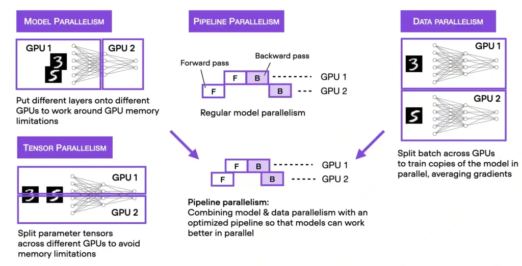
We will start with the simplest technique, data parallelism via DistributedDataParallel. Using the Trainer, we only have to modify one line of code:
        trainer = L.Trainer(
            max_epochs=3,
            callbacks=callbacks,
            accelerator="gpu",
            devices=4,  # <-- NEW
            strategy="ddp",  # <-- NEW
            precision="16",
            logger=logger,
            log_every_n_steps=10,
            deterministic=True,
        )
On my computer, with four A100 GPUs, this code ran in 3.07 min, reaching a test accuracy of 93.1%. Again, the test set improvement is likely due to the gradient averaging when using the data parallelism.

(Explaining data parallelism in detail is another great topic for a future article.)

6) DeepSpeed
Lastly, let us explore the DeepSpeed multi-GPU strategies we can use from within the Trainer.
But before trying it out in practice, l wanted to share my multi-GPU usage recommendations. Which strategy to use largely depends on the model, the number of GPUs, and the memory size of the GPUs. For example, when pretraining large models where the model does not fit on a single GPU, it’s a good idea to start with the simple "ddp_sharded” strategy, which adds tensor parallelism to "ddp". Using the previous code, "ddp_sharded" takes 2.58 min to run.
Alternatively, we can also consider the more sophisticated "deepspeed_stage_2" strategy, which shards the optimizer states and gradients. If this is not enough to fit the model into GPU memory, try the "deepspeed_stage_2_offload" variant, which offloads optimizer and gradient states to CPU memory (at a performance cost). You can find more information about the DeepSpeed strategies and their ZeRO (zero-redundancy optimizer) in the official ZeRO tutorial—furthermore, see the ZeRO offload tutorial for more information about offloading.
Returning to the recommendations, if you want to finetune a model, computational throughput is usually less of a concern than being able to fit the model into the memory of a smaller number of GPUs. In this case, you can explore the "stage_3" variants of deepspeed, which shard everything, optimizers, gradients, and parameters, i.e.
strategy="deepspeed_stage_3"strategy="deepspeed_stage_3_offload"
Since GPU memory is not a concern with a small model like DistilBERT, let’s try out "deepspeed_stage_2":
First, we have to install the DeepSpeed Python library:
pip install -U deepspeed(On my machine, this installed deepspeed-0.8.2.)
Next, we can enable "deepspeed_stage_2" with changing only one line of code:
        trainer = L.Trainer(
            max_epochs=3,
            callbacks=callbacks,
            accelerator="gpu",
            devices=4,
            strategy="deepspeed_stage_2",  # <-- NEW
            precision="16",
            logger=logger,
            log_every_n_steps=10,
            deterministic=True,
        )
This took 2.75 min to run on my machine and achieved 92.6% test accuracy.
Note that PyTorch now also has its own alternative to DeepSpeed, called fully-sharded DataParallel, which we can use via strategy="fsdp".

7) Fabric
With the recent Lightning 2.0 release, Lightning AI released the new Fabric open-source library for PyTorch. Fabric is essentially an alternative way to scale PyTorch code without using the LightningModule and Trainer I introduced above in section 2) Using the Trainer Class.
Fabric only requires changing a few lines of code, as shown in the code below. The - indicate lines that were removed and + were the lines that were added to convert the Python code to use Fabric.
    import os
    import os.path as op
    import time

    + from lightning import Fabric

    from datasets import load_dataset
    import matplotlib.pyplot as plt
    import pandas as pd
    import torch
    from torch.utils.data import DataLoader
    import torchmetrics
    from transformers import AutoTokenizer
    from transformers import AutoModelForSequenceClassification
    from watermark import watermark

    from local_dataset_utilities import download_dataset, load_dataset_into_to_dataframe, partition_dataset
    from local_dataset_utilities import IMDBDataset


    def tokenize_text(batch):
        return tokenizer(batch["text"], truncation=True, padding=True)


    def plot_logs(log_dir):
        metrics = pd.read_csv(op.join(log_dir, "metrics.csv"))

        aggreg_metrics = []
        agg_col = "epoch"
        for i, dfg in metrics.groupby(agg_col):
            agg = dict(dfg.mean())
            agg[agg_col] = i
            aggreg_metrics.append(agg)

        df_metrics = pd.DataFrame(aggreg_metrics)
        df_metrics[["train_loss", "val_loss"]].plot(
            grid=True, legend=True, xlabel="Epoch", ylabel="Loss"
        )
        plt.savefig(op.join(log_dir, "loss.pdf"))

        df_metrics[["train_acc", "val_acc"]].plot(
            grid=True, legend=True, xlabel="Epoch", ylabel="Accuracy"
        )
        plt.savefig(op.join(log_dir, "acc.pdf"))


    - def train(num_epochs, model, optimizer, train_loader, val_loader, device):
    + def train(num_epochs, model, optimizer, train_loader, val_loader, fabric):

          for epoch in range(num_epochs):
    -         train_acc = torchmetrics.Accuracy(task="multiclass", num_classes=2).to(device)
    +         train_acc = torchmetrics.Accuracy(task="multiclass", num_classes=2).to(fabric.device)

            model.train()
            for batch_idx, batch in enumerate(train_loader):

    -             for s in ["input_ids", "attention_mask", "label"]:
    -                 batch[s] = batch[s].to(device)

                outputs = model(batch["input_ids"], attention_mask=batch["attention_mask"], labels=batch["label"])
                optimizer.zero_grad()
    -            outputs["loss"].backward()
    +            fabric.backward(outputs["loss"])

                ### UPDATE MODEL PARAMETERS
                optimizer.step()

                ### LOGGING
                if not batch_idx % 300:
                    print(f"Epoch: {epoch+1:04d}/{num_epochs:04d} | Batch {batch_idx:04d}/{len(train_loader):04d} | Loss: {outputs['loss']:.4f}")

                model.eval()
                with torch.no_grad():
                    predicted_labels = torch.argmax(outputs["logits"], 1)
                    train_acc.update(predicted_labels, batch["label"])

            ### MORE LOGGING
            model.eval()
            with torch.no_grad():
    -            val_acc = torchmetrics.Accuracy(task="multiclass", num_classes=2).to(device)
    +            val_acc = torchmetrics.Accuracy(task="multiclass", num_classes=2).to(fabric.device)
                for batch in val_loader:
    -                for s in ["input_ids", "attention_mask", "label"]:
    -                    batch[s] = batch[s].to(device)
                    outputs = model(batch["input_ids"], attention_mask=batch["attention_mask"], labels=batch["label"])
                    predicted_labels = torch.argmax(outputs["logits"], 1)
                    val_acc.update(predicted_labels, batch["label"])

                print(f"Epoch: {epoch+1:04d}/{num_epochs:04d} | Train acc.: {train_acc.compute()*100:.2f}% | Val acc.: {val_acc.compute()*100:.2f}%")
                train_acc.reset(), val_acc.reset()


    if __name__ == "__main__":

        print(watermark(packages="torch,lightning,transformers", python=True))
        print("Torch CUDA available?", torch.cuda.is_available())
    -   device = "cuda" if torch.cuda.is_available() else "cpu"
        torch.manual_seed(123)

        ##########################
        ### 1 Loading the Dataset
        ##########################
        download_dataset()
        df = load_dataset_into_to_dataframe()
        if not (op.exists("train.csv") and op.exists("val.csv") and op.exists("test.csv")):
            partition_dataset(df)

        imdb_dataset = load_dataset(
            "csv",
            data_files={
                "train": "train.csv",
                "validation": "val.csv",
                "test": "test.csv",
            },
        )

        #########################################
        ### 2 Tokenization and Numericalization
        #########################################

        tokenizer = AutoTokenizer.from_pretrained("distilbert-base-uncased")
        print("Tokenizer input max length:", tokenizer.model_max_length, flush=True)
        print("Tokenizer vocabulary size:", tokenizer.vocab_size, flush=True)

        print("Tokenizing ...", flush=True)
        imdb_tokenized = imdb_dataset.map(tokenize_text, batched=True, batch_size=None)
        del imdb_dataset
        imdb_tokenized.set_format("torch", columns=["input_ids", "attention_mask", "label"])
        os.environ["TOKENIZERS_PARALLELISM"] = "false"

        #########################################
        ### 3 Set Up DataLoaders
        #########################################

        train_dataset = IMDBDataset(imdb_tokenized, partition_key="train")
        val_dataset = IMDBDataset(imdb_tokenized, partition_key="validation")
        test_dataset = IMDBDataset(imdb_tokenized, partition_key="test")

        train_loader = DataLoader(
            dataset=train_dataset,
            batch_size=12,
            shuffle=True,
            num_workers=2,
            drop_last=True,
        )

        val_loader = DataLoader(
            dataset=val_dataset,
            batch_size=12,
            num_workers=2,
            drop_last=True,
        )

        test_loader = DataLoader(
            dataset=test_dataset,
            batch_size=12,
            num_workers=2,
            drop_last=True,
        )


        #########################################
        ### 4 Initializing the Model
        #########################################

    +    fabric = Fabric(accelerator="cuda", devices=4,
    +                    strategy="deepspeed_stage_2", precision="16-mixed")
    +    fabric.launch()

        model = AutoModelForSequenceClassification.from_pretrained(
            "distilbert-base-uncased", num_labels=2)

    -   model.to(device)
        optimizer = torch.optim.Adam(model.parameters(), lr=5e-5)

    +    model, optimizer = fabric.setup(model, optimizer)
    +    train_loader, val_loader, test_loader = fabric.setup_dataloaders(
    +        train_loader, val_loader, test_loader)

        #########################################
        ### 5 Finetuning
        #########################################

        start = time.time()
        train(
            num_epochs=3,
            model=model,
            optimizer=optimizer,
            train_loader=train_loader,
            val_loader=val_loader,
    -       device=device
    +       fabric=fabric
        )

        end = time.time()
        elapsed = end-start
        print(f"Time elapsed {elapsed/60:.2f} min")

        with torch.no_grad():
            model.eval()
    -       test_acc = torchmetrics.Accuracy(task="multiclass", num_classes=2).to(device)
    +       test_acc = torchmetrics.Accuracy(task="multiclass", num_classes=2).to(fabric.device)
            for batch in test_loader:
    -           for s in ["input_ids", "attention_mask", "label"]:
    -               batch[s] = batch[s].to(device)
                outputs = model(batch["input_ids"], attention_mask=batch["attention_mask"], labels=batch["label"])
                predicted_labels = torch.argmax(outputs["logits"], 1)
                test_acc.update(predicted_labels, batch["label"])

        print(f"Test accuracy {test_acc.compute()*100:.2f}%")
As we can see, the modifications are really lightweight! How well does it run? Fabric completed the finetuning in just 1.8 min! Fabric is a bit more lightweight than the Trainer – although it’s capable using callbacks and logging as well, we haven’t enabled these features here to demonstrate Fabric with a minimalist example. It’s blazing fast, isn’t it?
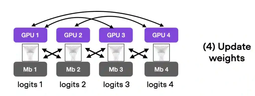
When to use the Lightning Trainer or Fabric depends on your personal preference. As a rule of thumb, if you prefer a light wrapper around existing PyTorch code, check out Fabric. On the other hand, if you move towards bigger projects and prefer the code organization that Lightning provides, I recommend the Trainer.
Conclusion
In this article, we explored various techniques to improve the training speed of PyTorch models. If we use the Lightning Trainer, we can toggle between these options with one line of code, which is very convenient – especially if you are toggling between a CPU and GPU machine when debugging your code.

