When it comes to solving classification problems, logistic regression is often the first algorithm that comes to our mind. The theoretical concepts of logistic regression are essential for understanding more advanced concepts in deep learning.

Lets get Started

Introduction:

Logistic regression is a fundamental classification algorithm used to predict the probability of categorical dependent variable.

The idea of logistic regression is to find the relationship between independent variables and the probability of dependent variables. Simply put, it is a classification algorithm used when the response variable is categorical typically binary (e.g. 0 or 1).

A Simple Example

Suppose you have patient data and want to predict whether a person is likely to be diagnosed with diabetes. The output is binary: either diagnosed (1) or healthy (0). Similarly:

• Will it rain today? (Yes or No)
• Is this email spam? (Yes or No)

Classification Problem (Image by the Author)

This type of problem is referred to as binary logistic regression or binomial logistic regression.After binary logistic regression, Logistic regression also has variants like:

• Multinomial Logistic Regression : When the response variable has three or more outcomes (e.g., predicting weather: sunny, rainy, or snowy).
• Ordinal logistic regression can be binary or multinomial outcomes but in order like rating, class ranking of student(Excellent, Average, Bad).

Now, that you have a pretty good idea of logistic regression, lets understand why we cant just use linear regression for these problems.

Why Not Just Use Linear Regression?

Why cant we use linear regression for binary outcomes? Great question!

Imagine trying to predict whether someone will buy a product or not (0 or 1).

Linear regression might give predictions like:

• 1.8 (Umm what does that mean? Theyre super likely to buy?)
• -0.3 (Negative probability? Thats not even possible!)

Logistic regression fixes this by introducing the sigmoid function;

This transforms the linear line into an S-shaped curve, which maps any value to the range [0, 1]. Pretty neat, right?

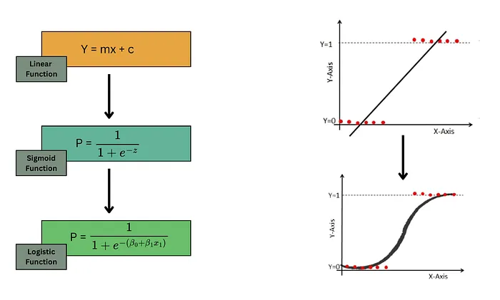
Logistic Function (Image by the Author)

Cost Function in Logistic Regression:

The goal of logistic regression is to find the best weights (parameters) that minimize the error. In linear regression, we use Mean Squared Error (MSE) as the cost function,

The graph of the cost function in linear regression:

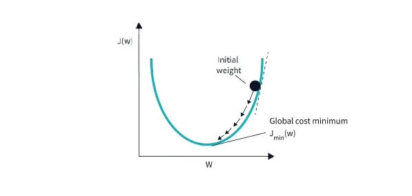
but for logistic regression, MSE doesnt work well. Why? Because the sigmoid function is nonlinear, MSE would result in a non-convex curve

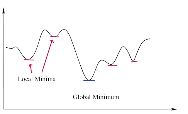
Image by the Author

A non-convex function has many local minimums which makes it very hard for the cost function to reach a global minimum and it increases the error rate as well.(oh no!).

Instead of MSE, we derive a different cost function known as the log-loss function or cross-entropy loss.

Now, we understand the whole scenario behind not using Linear regression. Lets understand gradient descent in Logistic regression and we minimize the error for the best performing model.

Gradient Descent is an optimization algorithm that is used to find the values of the parameters of a function (linear regression, logistic regression etc.) that is used to reduce a cost function. Check out this blog to get deeper understanding of Gradient Descent

Complete Mathematical Derivation of Logistic Function

Alright buckle-up, now were going to get mathematical

If youre familiar with calculus, youll get how the derivatives lead to these equation. But, if calculus isnt your thing, no worries just focus on understanding how it works intuitively, and thats more than enough to grasp whats happening behind the scenes.

And dont get confused over notations like w, or theyre just different ways of saying the same thing, commonly used in the literature.

Lets take a look at the logistic(sigmoid) function first:

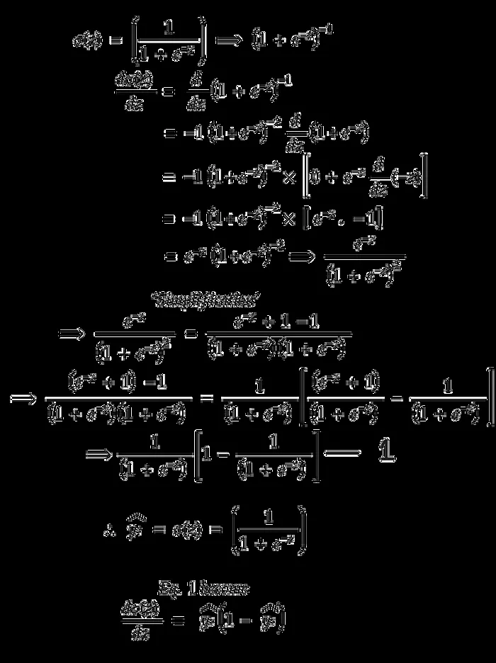
Step 1: Derivative of the Sigmoid Function

Before calculating the derivative of our cost function well first find a derivative for our sigmoid function because it will be used in the cost function.

Step 2: Compute the Gradient of the Cost Function

To minimize the cost function, we compute its gradient with respect to the weights w. The derivative of the cost function of a single data point:

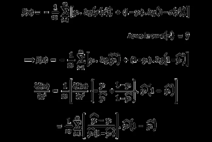
Step 3: Chain Rule to Compute J(w)/w:

Now, compute the gradient with respect to the weights . Using the chain rule, from step 1 and step 2:

Substitute:

Step 4: Weight Update

After the derivatives are calculated, Using gradient descent, we update the weights as follows equation:

Scale the step size by : Here **** is the learning rate that controls the updates from being too large (which could cause the algorithm to overshoot the minimum) or too small (which could make convergence very slow). Therefore, finding the optimal learning rate is crucial, and this is typically done through experimentation.

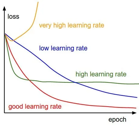
Source: Learning rate impact by cs231n

Alright! Take a look at weight update function again, You might have question whats the reason for subtracting old weights with derivatives to update.

Well, the idea is Gradient gives us the direction to reach the steepest ascent, subtraction is essential it ensures were moving against the gradient to minimize the cost function. If we added the gradient instead:

wed move toward the maximum of J(w), which is the opposite of what we want when minimizing.

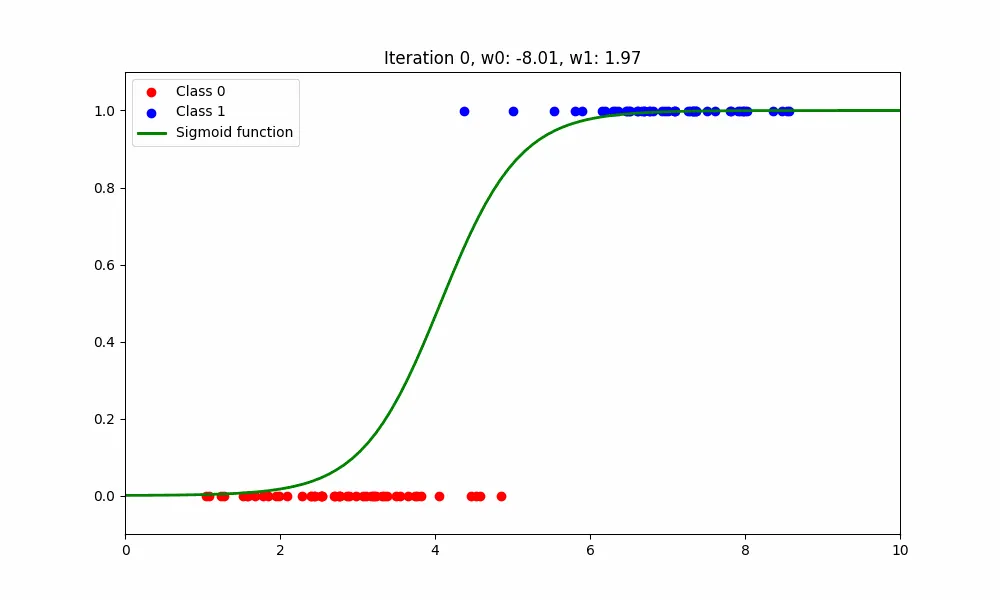
Since the gradient descent algorithm is an iterative approach, we first randomly take the values of weights and then change it such that the cost function becomes less and less until we reach at minima.

Enough math lets implement logistic regression step by step in Python!

Implementation in Python:

Well use the mathematical formulas derived above to build a logistic regression model from scratch.

Import numpy and Initialize the class:

     import numpy as np      class Logistic_Regression():        def __init__(self):          self.coef_ = None          self.intercept = None

2. Define the Sigmoid Function:

     def sigmoid(self, z):          
         return 1 / (1 + np.exp(-z))

3. Compute the Cost and Gradient:

     # Cost Function: -1/m [y_i * log() + (1 - y_i) * log(1 - )]         def cost_function(self, X, y, weights):          z = np.dot(X, weights)          predict_1 = y * np.log(self.sigmoid(z))          predict_2 = (1 - y) * np.log(1 - self.sigmoid(z))          return -sum(predict_1 + predict_2) / len(X)

Train Model:

     def fit(self, X, y, lr=0.01, n_iters=1000):              # Reason to add columns of ones at first, to include the intercept term in calculation as well (X.W)              X = np.c_[np.ones((X.shape[0], 1)), X]              # Initialize weights randomly              self.weights = np.random.rand(X.shape[1])              # To track the loss over iterations              losses = []                    for _ in range(n_iters):                  # Compute predictions                  z = np.dot(X, self.weights)                  y_hat = self.sigmoid(z)                        # Compute gradient                  gradient = np.dot(X.T, (y_hat - y)) / len(y)                        # Update weights                  self.weights -= lr * gradient                        # Track the loss                  loss = self.cost_function(X, y, self.weights)                  losses.append(loss)                    self.coef_ = self.weights[1:]                self.intercept_ = self.weights[0]

5. Make Predictions:

     def predict(self, X):          X = np.c_[np.ones((X.shape[0], 1)), X]          z = np.dot(X, self.weights)          predictions = self.sigmoid(z)          return [1 if i > 0.5 else 0 for i in predictions]

Heres the complete code on Github

Conclusion:

And thats it for this blog!

In this blog, weve walked through logistic regression, explored the math behind it, and built our own model from scratch in Python. Pretty cool!!

Logistic regression is a fundamental classification algorithm, and understanding its concepts is super important for stepping into deep learning.